Speculative Decoding: How Draft-Model Parallelism Cuts LLM Inference Latency
Large language model inference is slow for a counterintuitive reason: the GPU is mostly idle. At low batch sizes, each decoding step is memory-bandwidth-bound — the model’s weights stream from HBM to SRAM, the arithmetic units do a tiny amount of work for one token, then wait for the next weight load. Model FLOP-s Utilization during decoding is typically below 10%. The compute cores sit idle 90% of the time.
Speculative decoding exploits this idle compute with an elegant two-model trick: a small, fast draft model cheaply proposes K candidate tokens, and the large target model verifies all K in a single forward pass. Because the weights are loaded once regardless of how many tokens are processed, verifying K tokens fills that idle compute almost for free. When the draft guesses well, one target forward pass yields K+1 tokens instead of 1. When it guesses poorly, the worst case is no slower than ordinary decoding.
But the speedup is narrowly conditional. It requires the target to be memory-bandwidth-bound (small batch), the draft to agree often with the target (high acceptance), and the verification overhead to stay near-constant. At large batch sizes the target becomes compute-bound, the “free” verification stops being free, and speculative decoding can make inference slower. Production measurements show 2–3.55× speedups at batch size 1 collapsing to below 1.0× by batch 64–128 on dense models.
This is the story of a technique with a beautiful mathematical guarantee, a powerful but narrow hardware exploit, and a variant landscape where no one has done a fair head-to-head comparison.
The four-phase loop
Speculative decoding runs a four-phase loop each iteration [1][2]:
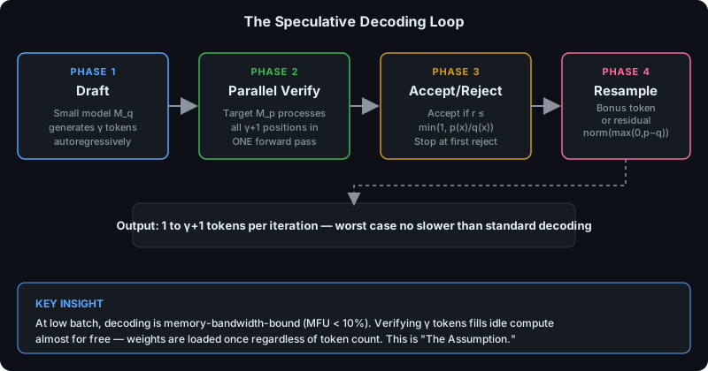
Figure 1 — The four-phase speculative decoding loop. The key exploit is Phase 2: verifying γ tokens in one forward pass costs roughly the same as generating one token, because the model weights are loaded once regardless of token count.
-
Draft. A small draft model
M_qautoregressively generates γ candidate tokensx₁, …, x_γ, one at a time. This costs γ sequential forward passes of the small model — cheap because the model is small. -
Parallel verification. The target model
M_pprocesses the full sequence [prefix, x₁, …, x_γ] in a single forward pass, producing probability distributionsp₁(x), …, p_{γ+1}(x)for all γ+1 positions at once. This is the central exploit: verifying γ tokens costs roughly the same wall-clock time as generating one. -
Accept/reject. For each draft token
x_i, drawr_i ~ Uniform(0,1)and accept ifr_i ≤ min(1, p_i(x_i)/q_i(x_i)). Stop at the first rejection; later tokens were conditioned on the rejected one and are discarded. -
Resample or bonus. If all γ tokens were accepted, sample a bonus token from
p_{γ+1}(x)— free, because the target already computed it. If token i was rejected, resample from the residual distributionp'(x) = norm(max(0, p_i(x) − q_i(x))).
Each iteration produces between 1 and γ+1 tokens. The worst case — immediate rejection — is no slower than standard autoregressive decoding. [1][2][3]
Why one forward pass can verify γ tokens
The hardware argument is precise. Standard autoregressive decoding at low batch sizes is memory-bandwidth-bound, not compute-bound. Each step loads the entire model weights from HBM to produce a single token. The GPU’s arithmetic units sit idle waiting for memory transfers.
Verifying γ+1 tokens in one forward pass adds compute but barely adds memory traffic, because:
- MLP layers: the linear weight matrices dominate, and they are loaded once whether processing 1 token or γ+1 tokens.
- Attention layers: the KV cache is loaded once regardless of how many new tokens are verified.
- Activations: at small batch and small γ, activation communication is latency-bound, not throughput-bound, so cost is similar for 1 or γ+1 tokens.
Chen et al. state this precisely: “the latency of parallel scoring of short continuations…is comparable to that of sampling a single token from the larger target model.” [2] Call this The Assumption — it is the load-bearing hardware premise, and it breaks when the target becomes compute-bound (high batch) or for MoE models where more tokens can activate more experts. [1][6]
The acceptance criterion and why it is exact
For each draft token x_i, accept with probability:
α(x_i) = min(1, p(x_i) / q(x_i))
where p is the target probability and q the draft probability. Two cases:
- p(x) ≥ q(x): always accept. The target wants this token more than the draft proposed it.
- p(x) < q(x): accept with probability
p(x)/q(x) < 1. The draft over-proposed this token; reject some instances to correct its frequency.
On rejection, sample from the residual distribution:
p’(x) = max(0, p(x) − q(x)) / Σ_x’ max(0, p(x’) − q(x’))
This captures exactly the probability mass where the target exceeds the draft — the “missing mass” the acceptance step failed to generate.
The proof of exactness
This is the part that makes speculative decoding remarkable: the output distribution is exactly the target model’s distribution, not approximately. For any token x', the total probability of producing it is the sum of accepting it and rejecting-then-resampling it:
P(accept x') = q(x') · min(1, p(x')/q(x')) = min(q(x'), p(x'))P(reject, x = x') = (1 − β) · p'(x') = p(x') − min(q(x'), p(x'))
Summing: P(x = x') = min(q, p) + p(x') − min(q, p) = p(x').
This holds for any distributions p and q — even an n-gram model, a random predictor, or a different architecture. The output is exactly distributed as the target, not approximately. [1][2][4][7] Three independent derivations — Leviathan et al. (Appendix A.1) [1], Brenndoerfer [4], and philkrav [6] — and Chen et al.’s Theorem 1 [2] all reach the identical result.
Acceptance rate equals 1 minus total variation distance
Leviathan et al. (Theorem 3.5) prove the per-token acceptance probability is:
α = E[β] = Σ_x min(p(x), q(x)) = 1 − TVD(p, q)
where TVD(p, q) = Σ_x |p(x) − q(x)| / 2 is the total variation distance. [1] Identical models give TVD = 0, α = 1, every draft token accepted. Disjoint support gives TVD = 1, α = 0, every token rejected, no speedup.
Theoretical speedup
Under an i.i.d. simplification, the walltime-improvement factor (Theorem 3.8 [1]), with cost coefficient c = t_draft / t_target:
E(speedup) = (1 − α^{γ+1}) / [(1 − α)(γc + 1)]
Bounded above by γ+1 (when α → 1 and c → 0). If α > c, speculative decoding always provides a speedup for some γ. philkrav generalizes with a batch-overhead term β: when β ≈ 1 (memory-bound), this reduces to Theorem 3.8; when β → γ+1 (compute-bound), speedup → 1 and there is no benefit. [6]
Optimality
Yin et al. 2024 (Theorem 2) prove that no unbiased rejection-based algorithm can have fewer expected rejections than standard speculative decoding. [7] The specific choices b_t = min(1, q_t/p_t) and P_t = [q_t − p_t]₊ are already optimal — improving the rejection rate requires sacrificing distribution preservation, using multiple parallel draft sequences, or using extra information beyond the models’ distributions.
Common misconceptions
| Misconception | Reality |
|---|---|
| ”It just samples from the draft model.” | Output is exactly the target distribution. The draft only proposes; the target verifies or resamples. |
| ”It’s an approximation.” | Mathematically exact: P(output = x') = p(x') for every token. |
| ”Accept when both models agree.” | The criterion is a ratio test, not an agreement test. When p ≥ q, always accept even if “different." |
| "On rejection, re-run the draft.” | Resample from the residual norm(max(0, p−q)), not from q. |
| ”It always speeds things up.” | Requires memory-bound target, high acceptance, low verification overhead. It can slow down inference. |
| ”The draft must be a smaller version.” | Correctness holds for any q — even an n-gram model. A bigram model achieves α ≈ 0.2 on translation. |
When the speedup is real vs illusory
Speculative decoding trades extra compute for reduced wall-clock latency. This is a net win only when the target is memory-bandwidth-bound — i.e., underutilized. Once the target is compute-saturated, the “free” verification becomes real work, and the speedup disappears or reverses.
Batch size is the master variable
Production measurements converge on a clear pattern: big speedups at batch 1, collapse by batch 64–128 on dense models.
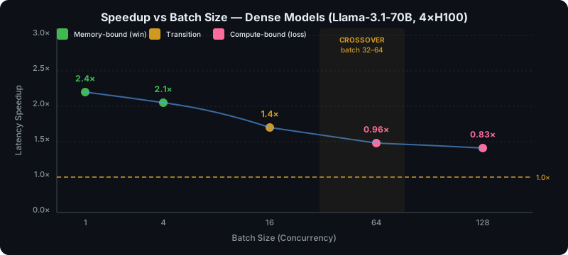
Figure 2 — Speedup vs batch size on Llama-3.1-70B (4×H100). The crossover where speedup falls below 1.0× sits between batch 32 and 64. Below the dashed line, speculative decoding makes inference slower.
| Concurrency | Baseline TPOT | Spec TPOT | Latency Speedup |
|---|---|---|---|
| 1 | 44 ms | 18 ms | 2.4× |
| 4 | 46 ms | 22 ms | 2.1× |
| 16 | 52 ms | 38 ms | 1.4× |
| 64 | 72 ms | 75 ms | 0.96× (slower) |
| 128 | 120 ms | 145 ms | 0.83× (slower) |
Llama-3.1-70B, 4×H100, with draft model. [4]
NVIDIA’s batch-size-1 TensorRT-LLM benchmarks on H200 with Llama 3.3 70B (FP8): 3.55× with a 1B draft, 3.16× with a 3B draft, 2.63× with an 8B draft. [12] The vLLM blog confirms the other direction: at high QPS, draft-model SD showed a 1.4× slowdown on ShareGPT and a 1.8× slowdown on CNN/DailyMail. [13]
The SpecDecode-Bench study — the first systematic sweep on production vLLM v0.10.1.1, H100, batch 1–128 — found the crossover where speedup falls below 1.0× sits between batch 32 and 64 for dense models. Tree-style verification (k=21) fell below 1.0× by batch 64 on all workloads; chain-style (k=3) stayed above 1.0× throughout. [11]
Long context changes the equation
The MagicDec paper (ICLR 2025) identifies a second regime: for long sequences, the bottleneck shifts from model-parameter loading (memory-bound at small batch) to KV-cache loading (memory-bound at large batch + long context). Because KV-cache size scales with batch × sequence length, and GPUs have a high FLOPS-to-bandwidth ratio, KV loading time grows faster than compute time as batch increases for long sequences. The result: above a critical sequence length S_inflection (~4,000 tokens for LLaMA-3.1-8B on 8×A100), SD speedup increases with batch size — up to 2.51× at batch 32–256. [20]
MoE models break the batch rule
Red Hat’s benchmarks of gpt-oss-120B (MoE, MXFP4) with EAGLE-3 on a single H200 showed speculative decoding improved throughput across all concurrency levels from 1 to 200: +20.7% throughput and +20.3% latency improvement on ShareGPT, +20.5% on SWE-bench, with a 19.4% cost reduction per million output tokens at peak. [16]
MoE models activate only a subset of experts per token, keeping active FLOPs low even at high batch — so they stay memory-bound longer. This contradicts the conventional wisdom that SD only helps at low concurrency, but has not been independently replicated on dense models.
Acceptance rate is the single most predictive metric
Below ~50% acceptance, speculative decoding is a net negative; above ~70%, it delivers strong speedups. [14] Typical acceptance rates from production data:
| Main Model | Draft Model | Acceptance Rate |
|---|---|---|
| Llama-3-70B | Llama-3-8B | ~65–75% |
| Llama-3-70B | Llama-3.2-1B | ~60–70% |
| Llama-3.1-405B | Llama-3.1-70B | ~70–80% |
Red Hat found that going from 3 to 4 draft tokens on gpt-oss-120B caused an 8% throughput regression because the extra draft token was rejected more often than not (acceptance dropped from 35.6% to 28.3%). [16]
Workload sensitivity
The speedup is highly task-dependent:
- Code generation (best): up to 90% faster p50 on Qwen 2.5 Coder 14B + 0.5B draft. [15]
- Chat (good): 1.5–2.8× at low batch on ShareGPT. [13]
- Summarization (good): 2.8× on CNN/DailyMail with n-gram (output overlaps input). [13]
- Reasoning (moderate): 1.64–1.80× on GPQA-Main; longer chains help. [11]
- Open-ended / creative (worst): no consistent benefit — draft diverges from target. [8]
- High temperature: hurts acceptance significantly. [14]
Dynamic speculative decoding is the production answer: systems (vLLM, TensorRT-LLM) adaptively shorten or disable speculation when load is high, queue depth is large, or acceptance drops. [13][14]
The variant landscape
Several variants attack different bottlenecks but inherit the same fundamental regime-dependence.
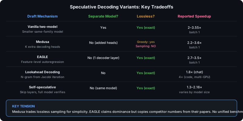
Figure 3 — The variant landscape. Each trades different bottlenecks — separate model, added heads, n-grams, layer skipping — but all inherit the same regime-dependence on batch size and acceptance rate.
Medusa adds K extra single-layer-MLP heads to the target model, each predicting tokens at a different offset, and verifies multiple candidate continuations simultaneously via tree attention. Two training variants: Medusa-1 (frozen backbone, ~2.2×) and Medusa-2 (joint training, 2.3–3.6× but requires a special recipe to preserve quality). Critically, Medusa’s “typical acceptance” scheme uses entropy-based thresholds rather than rigorous rejection sampling, so it is lossy in non-greedy settings. [21]
EAGLE predicts second-to-top-layer features (hidden states before the LM head) rather than tokens directly, reusing the target’s embedding layer and LM head. Its key innovation is incorporating the sampled token advanced by one time step to resolve feature-prediction uncertainty. EAGLE adds only ~0.24B params for a 7B model and uses rigorous speculative sampling, guaranteeing exactness for both greedy and non-greedy settings. It claims 2.7–3.5× for LLaMA2-Chat 70B and reports being 1.7–2.1× faster than Lookahead and 1.5–1.6× faster than Medusa on MT-bench. [22]
Lookahead Decoding reformulates autoregressive decoding as Jacobi iteration on a nonlinear system, maintains a 2D window (lookahead W × lookback N), caches n-grams from the Jacobi trajectory, and verifies candidates in parallel. No draft model, no training, no extra memory. Up to 1.8× on MT-bench and 4× on code completion with multi-GPU lookahead parallelism — but primarily effective in greedy decoding. [23]
Self-speculative / LayerSkip uses the target model itself as the drafter by skipping intermediate layers, then verifies with the full model. “Draft & Verify” (Zhang et al., ACL 2024) is plug-and-play with no training (up to 1.99×). LayerSkip (Elhoushi et al., ACL 2024, Meta) adds a training recipe (layer dropout + early exit loss) and reaches up to 2.16×. HuggingFace benchmarks show self-speculative beats two-model SD for most model sizes (Llama3 8B: 1.83× vs 1.53×) but loses for Llama2 70B (2.06× vs 2.83× with TinyLlama draft). [24][25][26]
Where the sources disagree
The MoE paradox
The SpecDecode-Bench study (dense models only) found speedup consistently degrades with batch size, falling below 1.0× by batch 64–128. Red Hat’s gpt-oss-120B (MoE) benchmarks showed +20% throughput even at 200 concurrent requests. These are not contradictory — they reflect a fundamental architectural difference. Dense models saturate compute as batch grows; MoE models activate only a subset of experts per token, keeping active FLOPs low and the model memory-bound for longer. The resolution: the batch-size rule applies to dense models; MoE models are a different regime. Practitioners should test their specific architecture rather than generalize.
EAGLE’s head-to-head validity
EAGLE’s claim to dominate Medusa and Lookahead rests on numbers copied from those papers’ own reports, run under different conditions. [22] The EAGLE paper itself states it copies Medusa and Lookahead speedup numbers “from their original technical reports” rather than re-running them under identical conditions. The comparison is conducted at batch size 1, greedy decoding, on MT-bench — excluding non-greedy settings entirely. Until an independent third party benchmarks all variants under unified conditions (same hardware, model, batch, task, temperature), the ranking is suggestive, not definitive.
The “free verification” assumption
Every speedup formula assumes verifying γ+1 tokens costs ≈ the same as generating 1 token. This is stated, not proven, in both original papers. [1][2] philkrav shows it breaks at batch size 2+ when implementations don’t fuse GEMM+dequant, and for MoE models where more tokens may activate more experts. [6] The assumption is a hardware-and-implementation fact, not a theorem, and its boundary is where the speedup lives or dies.
Devil’s advocate: the case that this is overstated
Recency bias toward vendor benchmarks. Many performance numbers come from NVIDIA, vLLM, Red Hat, Baseten, and Snowflake — all of whom have a commercial interest in showing their stack delivers big speedups. Vendor benchmarks almost always report the best-case configuration (batch 1, greedy, FP8, optimized kernel). The SpecDecode-Bench study is the most methodologically credible because it sweeps the full batch range — and it is also the source showing the smallest sustained speedups.
The “lossless” guarantee may be less meaningful than it sounds. The math proves the output distribution equals the target’s given the same random seed. In practice, floating-point non-determinism, different KV-cache layouts, and batch-dependent numerical behavior mean speculative-decoding outputs are bitwise different from non-speculative outputs even when statistically equivalent. “Lossless” is a distribution-level claim, not a bitwise claim — and some downstream evaluations (pass@1 on code) are sensitive to exact tokens.
The deployment-complexity tax is real. Each variant requires custom kernels (tree attention, feature prediction), draft-model management, and K tuning. In production, this complexity is a real cost that doesn’t appear in any speedup number. A team that deploys SD and gets 1.5× on a benchmark but 1.1× in production (due to integration overhead, scheduling interactions, memory pressure) has a legitimate complaint that the literature overstates practical gains.
The “MoE helps at high batch” finding rests on a single source. Red Hat’s gpt-oss-120B result is striking but unreplicated. If it turns out to be specific to that model’s expert configuration or quantization, the most exciting finding evaporates.
The optimality theorem is about rejection count, not wall-clock. Proving that standard speculative decoding minimizes expected rejections among unbiased algorithms does not prove it minimizes latency — because latency depends on the hardware regime, draft cost, and verification overhead, not just rejection count.
The honest read
Speculative decoding is a powerful latency optimization for interactive, low-batch, low-entropy workloads — not a universal throughput win. The math is beautiful: the rejection-sampling acceptance criterion is provably exact and provably optimal. The hardware exploit is real: at low batch, the GPU is 90% idle, and speculative decoding fills that idle compute. But the regime where both conditions hold — memory-bound target, high acceptance, low verification overhead — is narrow, and production serving systems that batch aggressively for throughput will often find themselves outside it.
The variant landscape is moving fast, with EAGLE-3, SWIFT, and other 2025–2026 methods publishing faster than any single report can track. The relative rankings are contested because no paper benchmarks competitors under identical conditions. The most credible independent benchmark — SpecDecode-Bench — shows the smallest sustained speedups and the clearest crossover points.
For practitioners: test your specific architecture, batch size, and workload. Don’t trust vendor benchmarks. Measure acceptance rate in production. Use dynamic speculative decoding that disables itself when the regime is wrong. And remember that the worst case is no slower than standard decoding — the downside is bounded, even if the upside is narrower than the papers suggest.
References
- Leviathan, Y., Kalman, M., & Matias, Y. (2023). “Fast Inference from Transformers via Speculative Decoding.” ICML 2023. proceedings.mlr.press/v202/leviathan23a.html — The original Google Research paper. Algorithm 1, correctness proof, acceptance-rate formula (Theorem 3.5: α = 1 − TVD), walltime-improvement formula (Theorem 3.8).
- Chen, C., Borgeaud, S., et al. (2023). “Accelerating Large Language Model Decoding with Speculative Sampling.” arXiv:2302.01318. arxiv.org/abs/2302.01318 — Concurrent DeepMind paper; same correctness guarantee; the observation that parallel scoring of K tokens has comparable latency to a single token.
- Mody, J. (2023). “Speculative Sampling.” jaykmody.com/blog/speculative-sampling/
- Brenndoerfer, M. “Speculative Decoding Math: Algorithms & Speedup Limits.” mbrenndoerfer.com
- Chen, J. “Deriving Speculative Sampling Intuitively.” jinghong-chen.net
- Kravchuk, P. (2024). “Speculative Decoding.” philkrav.com/posts/speculative/ — Generalized speedup formula with β (batch overhead); MoE analysis.
- Yin, M., Chen, M., et al. (2024). “A Theoretical Perspective for Speculative Decoding Algorithm.” NeurIPS 2024. arxiv.org/abs/2411.00841 — Optimality proof (Theorem 2).
- Leviathan, Y. “Looking back at speculative decoding.” Google Research Blog. research.google/blog
- NVIDIA. “An Introduction to Speculative Decoding.” developer.nvidia.com
- Sun, Z., et al. (2023). “SpecTr: Fast Speculative Decoding via Optimal Transport.” NeurIPS 2023. arxiv.org/abs/2310.15141
- SpecDecode-Bench. “Speculative Decoding: Performance or Illusion?” arxiv.org/html/2601.11580v2 — First systematic study on production vLLM; batch 1–128.
- NVIDIA TensorRT-LLM. “Boost Llama 3.3 70B Inference Throughput 3x.” developer.nvidia.com
- vLLM Blog. “How Speculative Decoding Boosts vLLM Performance by up to 2.8x.” vllm.ai/blog/2024-10-17-spec-decode
- Turion.ai. “Speculative Decoding for Production LLMs.” turion.ai
- Baseten. “How we built production-ready speculative decoding with TensorRT-LLM.” baseten.co
- Red Hat. “Performance improvements with speculative decoding in vLLM for gpt-oss.” developers.redhat.com
- Snowflake. “Fastest Speculative Decoding in vLLM with Arctic Inference.” snowflake.com
- AWS. “Accelerating decode-heavy LLM inference with speculative decoding on AWS Trainium.” aws.amazon.com
- NVIDIA. “N-Gram Speculative Decoding in TensorRT LLM.” nvidia.github.io
- MagicDec (ICLR 2025). “Breaking the Latency-Throughput Tradeoff for Long Context Generation.” arxiv.org/html/2408.11049v5
- Cai et al. (2024). “Medusa: Simple LLM Inference Acceleration Framework with Multiple Decoding Heads.” ICML 2024. arxiv.org/abs/2401.10774
- Li et al. (2024). “EAGLE: Speculative Sampling Requires Rethinking Feature Uncertainty.” ICML 2024. proceedings.mlr.press/v235/li24bt.html
- Fu et al. (2024). “Break the Sequential Dependency of LLM Inference Using Lookahead Decoding.” ICML 2024. arxiv.org/abs/2402.02057
- Zhang et al. (2024). “Draft & Verify: Lossless LLM Acceleration via Self-Speculative Decoding.” ACL 2024. arxiv.org/abs/2309.08168
- Elhoushi et al. (2024). “LayerSkip: Enabling Early Exit Inference and Self-Speculative Decoding.” ACL 2024. arxiv.org/abs/2404.16710
- HuggingFace Blog. “Faster Text Generation with Self-Speculative Decoding.” huggingface.co/blog/layerskip