The Inference Machine: KV Cache, Attention, and How Modern LLMs Stay Fast
The previous post covered how to read a model’s label — precision, format, architecture, fine-tune stage. This one covers what happens after you press send.
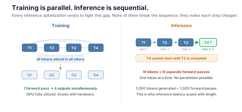
Training is embarrassingly parallel. Inference is not.
During training, you feed the model a batch of complete sentences. Every token attends to every other token simultaneously. The whole thing runs as a giant matrix multiplication across thousands of GPU cores at once. Fast.
During inference, you need to generate tokens one at a time. Each new token is conditioned on all previous tokens — but you can’t generate token 50 until you have token 49. The model is inherently sequential here. No matter how many GPUs you have, the fundamental clock of generation is: one token, then the next.
This distinction — parallel training, sequential inference — is the source of almost every optimization in modern LLM serving.
The attention bottleneck
The transformer’s attention mechanism works like this: for every token, compute three vectors — a Query (Q), a Key (K), and a Value (V). To figure out what a token should attend to, take its Query and compare it against the Keys of every other token. High similarity → attend more; low similarity → attend less. Then use those attention weights to blend the Values into the output.
The cost: computing K and V is expensive (large matrix multiplications, repeated across every layer), and comparing a Query against all previous Keys scales quadratically with sequence length. A 10× longer context is 100× more attention computation.
For a 1,000-token prompt that’s manageable. For a 1-million-token context window — where the frontier is heading — it’s a wall.
The fix: stop recomputing what you already have
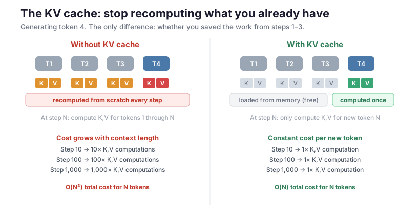
Here’s the key observation: if you’re generating token 50, you’ve already computed the Keys and Values for tokens 1–49. Those computations don’t change. So why throw them away?
The KV cache is the answer: store the K and V tensors for every previous token in GPU memory. When generating the next token, only compute K and V for that token, then reuse the cached values for everything before it.
It’s memoization — a pattern from 1968 computer science applied to 2024 neural networks. And it’s now the default behavior in every serious inference stack.
The practical impact: without KV cache, inference cost scales with sequence length squared. With it, you pay the full cost once on the prompt, and then each new token is roughly constant-time. That’s what makes long conversations usable.
The memory wall
KV cache solves the computation problem but creates a storage problem. The cache grows with every token: for a modern model with 32 attention layers, 16 heads, and BF16 precision, a single token occupies roughly 0.5 MB of KV cache. A 100K-token conversation: ~50 GB. A million tokens: 500 GB.
Nobody has 500 GB of GPU memory. And serving hundreds of simultaneous users, each with their own cache, multiplies the problem.
This is the memory wall — the bottleneck that explains why GPU memory bandwidth, not raw compute, determines how fast inference actually is. Every major architectural innovation since 2022 is at least partly a response to it.
How architectures responded
Multi-Head Attention → Multi-Query → Grouped-Query
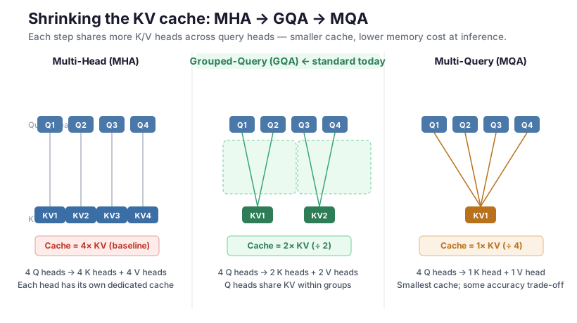
The simplest fix: don’t give every attention head its own separate K and V matrices. Share them.
- MQA (Shazeer, 2019): all query heads share a single K/V head. KV cache shrinks by up to 8×. Some accuracy loss.
- GQA (Ainslie et al., 2023): the middle ground — group query heads into clusters, each sharing one K/V head. Almost as small as MQA, almost as accurate as full MHA.
GQA is now the default in essentially every competitive open-weights model: Llama 3, Mistral, Qwen 3, Gemma 2. When a model card lists “grouped-query attention,” this is why.
Multi-Head Latent Attention (MLA)
DeepSeek went further. Instead of sharing heads, they compress the K and V matrices into a small latent vector at inference time, then decompress as needed. The KV cache stores the compressed form — a fraction the size of standard GQA — and accuracy holds. DeepSeek-V3’s near-frontier performance at low serving cost is largely MLA.
Mamba 2: a different premise
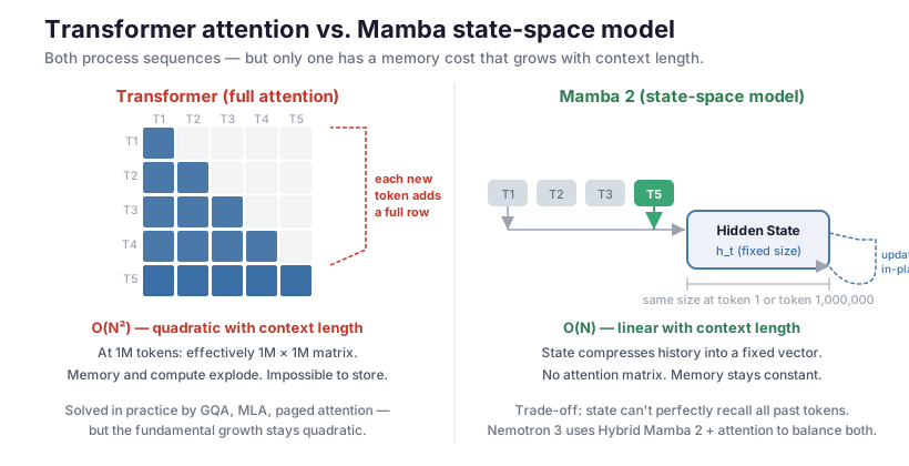
The approaches above all still have attention at their core. Mamba takes a different path: replace attention with a state-space model (SSM). Instead of comparing every token against every other, Mamba maintains a fixed-size hidden state that gets updated at each step — like a memory register. The cost is constant per token regardless of context length, not quadratic.
The catch: pure Mamba loses some of the recall quality you get from full attention. The state can’t hold everything. NVIDIA’s Nemotron 3 uses Hybrid Mamba 2: alternate Mamba 2 layers (constant-time, for most processing) with periodic full-attention layers (for precise recall when needed). The goal is linear-time scaling toward the 1M-token context window while preserving accuracy on tasks that require exact lookups.
PagedAttention
On the serving side, vLLM (Kwon et al., 2023) borrowed a trick from operating systems: instead of allocating a contiguous memory block for each request’s KV cache — which wastes memory badly when requests are different lengths — page the cache into fixed-size blocks, just like virtual memory. This reduced memory waste by up to 96% and doubled throughput on the same hardware.
Generating faster: multi-token prediction
Standard generation decodes one token per forward pass. Multi-token prediction (MTP) changes this: the model predicts the next several tokens in parallel during a single pass, then uses those predictions speculatively. If the guesses are right (and for fluent text they usually are), you’ve just generated multiple tokens for the cost of roughly one.
This is one half of speculative decoding — a technique that reduces wall-clock latency on capable hardware without changing output quality.
The sizing game: MoE and what active parameters actually mean
When Nemotron 3 ships a “550B total / 50B active” Ultra model, at inference time that means:
- All 550B parameters need to be loaded into memory (the router doesn’t know which experts it’ll need until it sees the token)
- The actual compute per token only involves ~50B parameters — the selected experts
- Decode speed feels like a 50B model; memory footprint feels like a 550B model
The three Nemotron 3 variants are explicitly sized to match NVIDIA’s GPU install base: consumer GPUs fit Nano’s ~30B total (nvfp4 cuts the effective footprint to ~15B), H100s fit Super’s 120B, and DGX clusters fit Ultra’s 550B.
This is the MoE bargain: speed is cheap, memory is not. The previous post covers this from the label side — a 35B-A3B model decodes fast but still loads heavy.
What this means for your prompt structure
KV cache and prompt caching have a direct consequence for how prompts should be structured in production:
Static content first, dynamic content last. Prompt caching works by hashing a prefix. If your system prompt, tool definitions, and reference documents sit at the top and change rarely, they can be cached and reused across requests. The user’s specific question — which changes every time — goes at the end.
The economics: a cached prefix can reduce input token costs by 80–90%. Anthropic’s prompt caching bills cached tokens at roughly a tenth of uncached; OpenAI applies it automatically for prefixes longer than 1024 tokens.
On-device, the same logic applies. Each new exchange in a long conversation is cheap because the history is in the KV cache. The expensive moment is when you clear it — starting a new conversation, or hitting the context limit and rolling the window.
Where to go deeper
In rough order of difficulty:
Papers
| Paper | Why it matters |
|---|---|
| ”Attention Is All You Need” (Vaswani et al., 2017) | Section 3.2 — the exact QKV math; where O(N²) comes from |
| ”One Write-Head is All You Need” (Shazeer, 2019) | Original MQA; short and clear |
| ”GQA: Training Generalized Multi-Query Models” (Ainslie et al., 2023) | Why every modern open-weights model uses GQA |
| ”Efficiently Scaling Transformer Inference” (Kwon et al., 2023) | PagedAttention and the vLLM serving system |
| DeepSeek-V3 Technical Report (2024) | MLA in detail; how they achieve frontier quality cheaply |
| ”Transformers are SSMs” (Dao & Gu, 2024) | The theory behind Mamba 2 and linear-time attention |
YouTube
- Adam Rosler — “KV Cache: The Invisible Trick Behind Every LLM”: the clearest visual walkthrough of auto-regressive decoding and why memoization fixes it. Start here.
- Caleb Writes Code — “NVIDIA’s Nemotron 3”: a good walkthrough of Hybrid Mamba 2 and the Nano/Super/Ultra sizing philosophy.
- Yannic Kilcher — “DeepSeek-V3”: the math of MLA latent compression explained at a deliberate pace.
- vLLM Deep Dive: PagedAttention, Continuous Batching & 24x Throughput: shows how the KV cache is managed across concurrent users at serving scale.
The model label tells you what a model costs to run. This post is about why it costs that. The KV cache is the connective tissue: it explains why context is priced by the token, why GQA is in every open-weights model, why Mamba 2 and MLA exist, and why your system prompt belongs at the top of every request. Once you see the bottleneck, the rest of the architecture decisions follow.